
Service Robot Fleet Right-Sizing: How Many Units Your Facility Actually Needs
At a glance: Fleet size is the number that decides whether a service robot deployment pays back or quietly loses money. Vendors quote units; what a facility buys is task-hours. This guide gives the arithmetic that converts floor area, shift structure and availability into a defensible unit count, and names the four assumptions that inflate quotes.

Why Unit Count Is the Wrong First Question
A procurement team receives a quote for six units and asks whether four would do. That question cannot be answered from the quote, because the quote was built from a floor area divided by a marketing coverage figure. The honest version of the question is: how many task-hours does this facility require per week, and how many productive hours does one unit deliver per week in this specific building?
Once the problem is stated in task-hours, fleet size stops being a negotiation and becomes arithmetic. Two facilities of identical square footage can need very different fleets, because the number is driven by route density, obstacle frequency, shift structure and door and elevator dwell time, not by area alone.
The Four Inputs You Need Before Any Number Is Meaningful
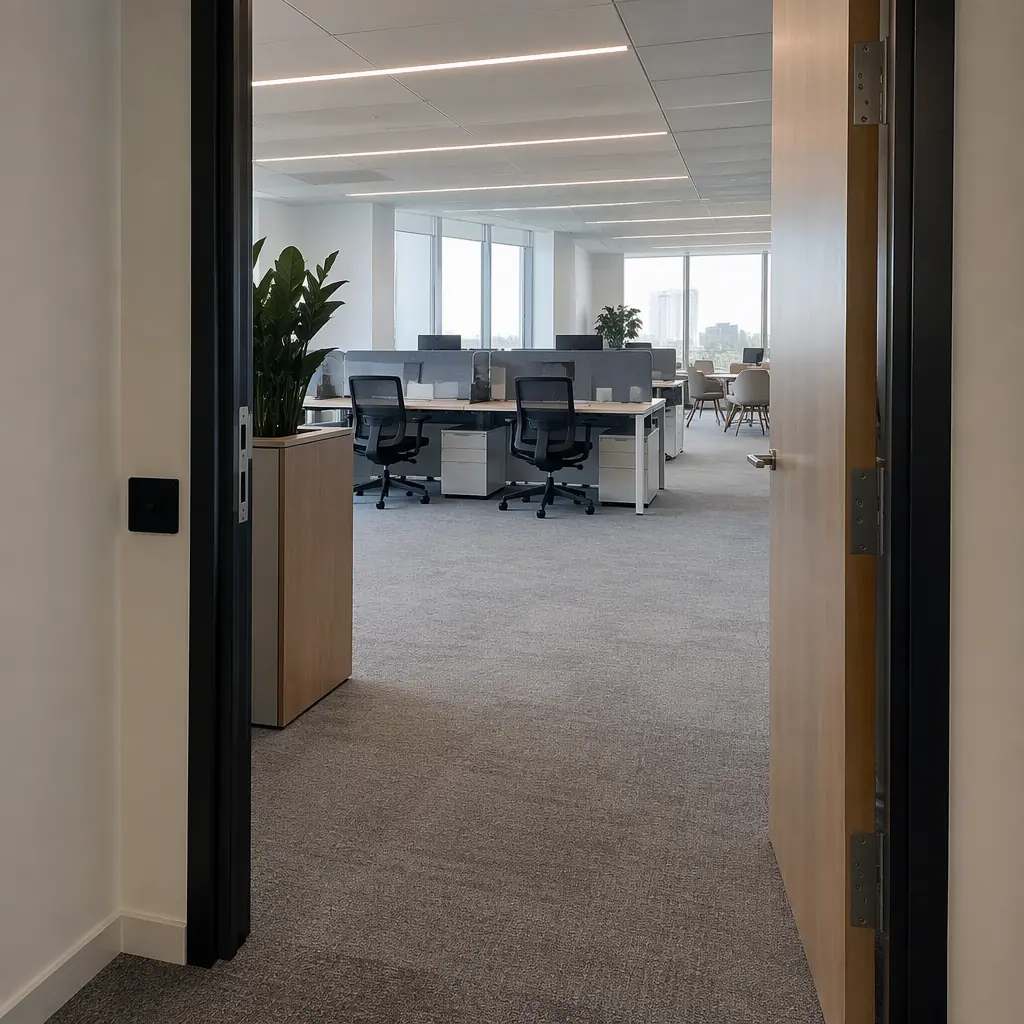
There are four inputs. Three come from your own operation and one comes from the vendor's engineering data. A vendor who cannot supply the fourth is guessing.
1. Required task-hours per period
Required task-hours is the cleanable or serviceable area multiplied by the labour minutes per unit area for that surface type, converted to hours. For a mixed facility you compute this per floor type, because hard floor, carpet and restroom work have very different per-area times. A 30,000 m² facility is not one workload; it is typically four or five workloads with different productivity rates.
2. Productive coverage rate for that surface, in this building
Productive coverage rate is the area a unit genuinely completes per hour, measured inside your building. It is always lower than the datasheet rate. Datasheet rates are measured on open, empty, regular floor with no turns around stacked chairs and no door transits. Published clean rate figures for large-format scrubbers sit in the range of 1,500 to 3,000 m² per hour; in dense, cluttered or multi-room environments, real throughput commonly lands 30% to 50% below that.
3. Availability factor
Availability is the fraction of scheduled operating hours the unit is actually able to work, after charging, maintenance, cleaning of the machine itself, and faults. A realistic planning figure for a well-supported fleet in a first year is 85% to 92%. Using 100% is the single most common cause of chronic under-delivery.
4. Peak concurrency requirement
Some buildings cannot spread work across the day. A retail floor that must be clean before 08:00 has a hard two-hour window, which sets a floor on unit count regardless of weekly arithmetic. Peak concurrency is often the binding constraint in retail and food service, and almost never the binding constraint in offices and warehouses.
The Sizing Formula, Step by Step
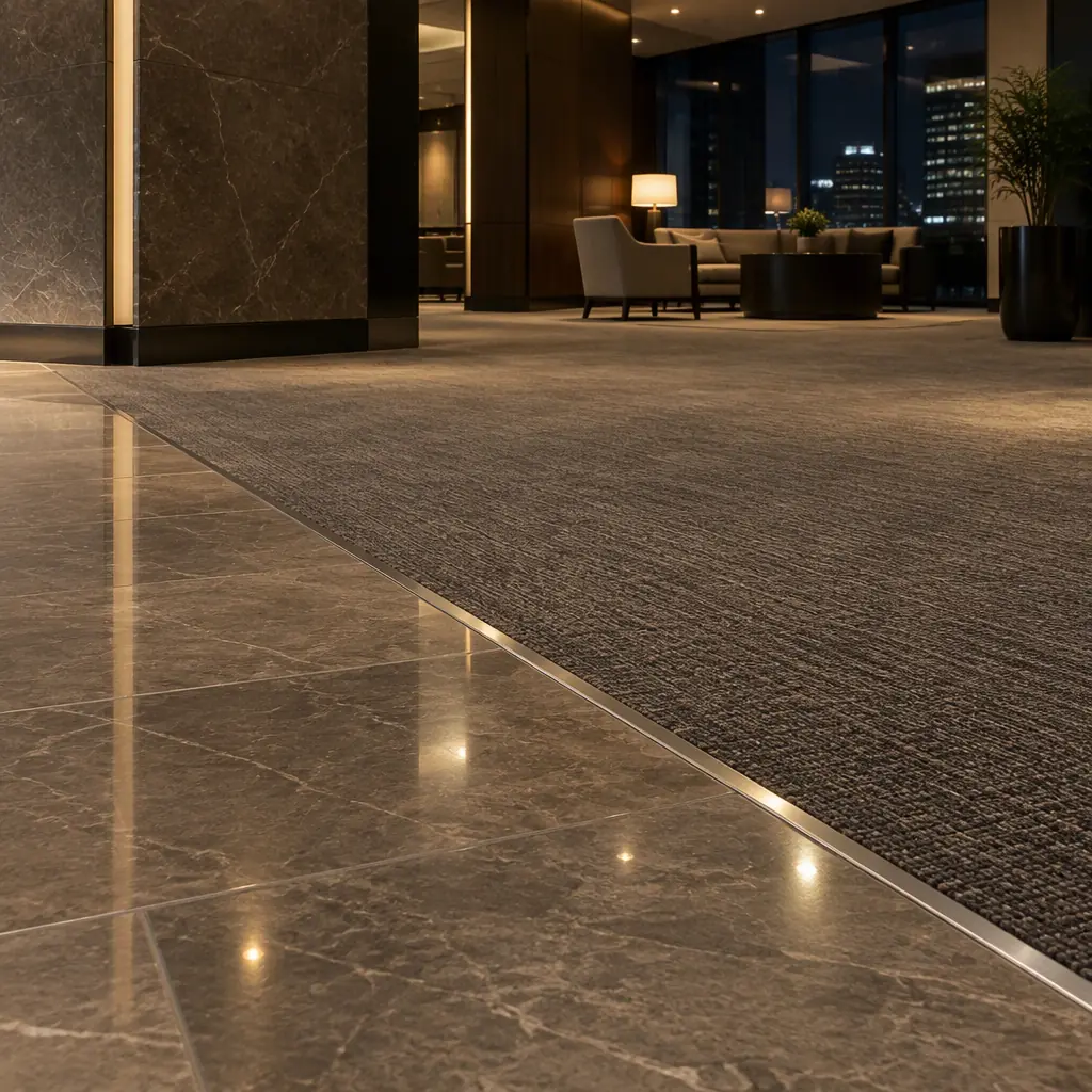
With those four inputs the calculation is short. Work it per surface type, then take the maximum across the shift structure and the peak-window constraint.
Step 1 — Compute weekly task-hours per surface type
Area divided by productive coverage rate gives hours per cleaning round. Multiply by rounds per week. A worked example for one facility:
| Surface type | Area | Productive rate | Rounds / week | Task-hours / week |
|---|---|---|---|---|
| Main lobby, polished stone | 4,200 m² | 1,900 m²/h | 14 | 31.0 |
| Open office, low-pile carpet | 18,000 m² | 1,100 m²/h | 5 | 81.8 |
| Corridors and stairs, hard floor | 6,300 m² | 1,700 m²/h | 7 | 25.9 |
| Restrooms and wet rooms | 1,500 m² | 350 m²/h | 14 | 60.0 |
| Canteen, hard floor | 2,000 m² | 1,400 m²/h | 12 | 17.1 |
| Total | 32,000 m² | 215.8 |
Step 2 — Convert to unit-hours using the availability factor
Divide total task-hours by the availability factor. At 88% availability, 215.8 task-hours requires 245.2 unit-hours of scheduled time. This is the number the fleet must be rostered against, not 215.8.
Step 3 — Divide by schedulable hours per unit per week
Schedulable hours is the operating window multiplied by days the site is open. A site operating a six-hour nightly window, six nights a week, offers 36 schedulable hours per unit. 245.2 divided by 36 gives 6.8 units, which rounds to 7. If the same site ran two six-hour windows across a longer operating day, the same task load would fit in 4 units plus one on maintenance rotation.
Step 4 — Apply the peak concurrency floor
Finally, check whether the peak window forces more units than the weekly arithmetic. If a 4,200 m² lobby must be finished inside a 90-minute pre-opening window, one unit at 1,900 m²/h needs 2.2 hours and therefore fails. Two units working in parallel complete it in 1.1 hours. The peak constraint sets a minimum of two even if the weekly load would suggest one.
The Four Errors That Double a Quote
Most oversized quotes trace back to one of four mistakes. Each is checkable before signature.
- Datasheet coverage rate used as productive rate. The 30% to 50% gap between published and in-building throughput is usually the largest single error. Insist that the vendor's rate is applied to your floor plan with your obstacle and door counts, and that the contract states a measured rate achieved during the pilot.
- Availability assumed at 100%. Charging time, filter and brush changes, water fills and firmware updates consume real hours. Planning at 88% is conservative and defensible.
- Every surface priced at hard-floor productivity. Restrooms and carpet dominate task-hours in almost every mixed facility. In the example above, restrooms are 4.7% of the area but 28% of the task-hours.
- Peak window ignored, then discovered in week one. A fleet sized on weekly arithmetic fails the first morning it meets a compressed window, and the emergency answer is overtime labour or extra units at list price.
A Right-Sizing Worksheet You Can Run in an Hour
The following table is the structure to fill in. Columns one to four come from your facility, column five is the vendor's contractual engineering figure.
| Item | Unit | Source | Example value |
|---|---|---|---|
| Cleanable area by surface type | m² | Floor plan / CAFM data | 32,000 |
| Rounds per week by surface | count | Cleaning specification | 5–14 |
| Productive coverage rate in building | m²/h | Vendor, validated in pilot | 1,100–1,900 |
| Availability factor | % | Planning assumption, contractually reported | 88% |
| Schedulable hours per unit per week | h | Operating window × operating days | 36 |
| Peak window requirement | m²/h | Opening-time constraint | 2,800 |
| Fleet size | units | max(weekly arithmetic, peak floor) | 7 |
Sizing for Redundancy Without Paying for It Twice
Fleet sizing and redundancy are different questions and should be budgeted separately. A fleet of seven units sized exactly to the weekly load has no spare capacity, and one unit down means the load either slips or moves to labour.
There are three ways to buy redundancy and they have different cost profiles. Buying a dedicated spare unit adds capital cost and a small amount of maintenance. Buying RaaS capacity with a contractual substitution right adds operating cost only when invoked. Cross-training two staff to cover specific routes during a fault adds neither, but it must be genuinely rehearsed rather than written into a plan.
For most single-site facilities under ten units, the substitution right is the cheapest redundancy, because it costs nothing on the days the fleet is healthy. For multi-site operators, pooling one spare across three or four sites is effective provided the sites are close enough for a same-day swap. Whichever route is chosen, the redundancy plan should appear in the fleet schedule and in the uptime definition, otherwise it exists only on paper.
How to Validate the Number Before You Commit Capital
Every input above can be tested at low cost before a purchase order. A two-week paid pilot on the two highest task-hour surface types produces a measured productive coverage rate and a measured availability figure. Substituting those two real numbers into the worksheet typically moves the fleet estimate by one to two units in either direction, which is generally larger than the price difference between vendors.
The pilot should be sized to stress the peak window specifically. A pilot that only runs in a quiet overnight window measures the easy case and will overstate coverable area. The most useful pilot data points are productive coverage rate on the hardest surface, the number of human interventions per shift, and the actual charging and maintenance hours consumed.
Once measured, the same figures become the performance clauses of the contract. A vendor asked to warrant an 88% availability factor and a stated coverage rate on a named surface is being asked a question it can answer. A vendor asked to warrant "industrial-grade performance" is not.
Putting It Together

Right-sizing is not a single calculation, it is a discipline of refusing to accept a unit count that cannot be derived. Four inputs, four steps, and one peak-window check produce a number you can defend to a finance committee and test in a pilot. The facilities that overspend on service robots almost never did the wrong arithmetic; they never did the arithmetic at all, and accepted a vendor's coverage figure as if it had been measured in their own building.